Shortcut functions

Single data set

The simplest way to compare two classifiers on a single data set is to call a function two_on_single.

baycomp.two_on_single(x, y, rope=0, runs=1, *, names=None, plot=False)

Compute probabilities using a Bayesian correlated t-test and, optionally, draw a histogram.

The test assumes that the classifiers were evaluated using cross validation. Argument runs gives the number of repetitions of cross-validation.

For more details, see CorrelatedTTest

Parameters:

• x (np.array) – a vector of scores for the first model
• y (np.array) – a vector of scores for the second model
• rope (float) – the width of the region of practical equivalence (default: 0)
• runs (int) – the number of repetitions of cross validation (default: 1)
• nsamples (int) – the number of samples (default: 50000)
• plot (bool) – if True, the function also return a histogram (default: False)
• names (tuple of str) – names of classifiers (ignored if plot is False)

Returns:

(p_left, p_rope, p_right) if rope > 0; otherwise (p_left, p_right).

If plot=True, the function also returns a matplotlib figure, that is, ((p_left, p_rope, p_right), fig)

Let nbc and j48 be numpy arrays with classification accuracies of naive Bayesian classifier and J48 obtained by cross-validation on some data set. Function two_on_single computes the probability that NBC is better than J48 and vice versa.

>>> two_on_single(nbc, j48)
(0.4145119975061462, 0.5854880024938538)

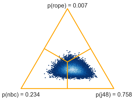
There is a 58.5 % probability that the average performance of J48 on this problem is better than that of NBC. We can add rope: let us consider the two methods equivalent if their classification accuracies differ by less than 0.5. (Recall again that rope is on the same scale as nbc and j48. If they are in percents, so is the rope.)

>>> two_on_single(nbc, j48, rope=0.5)
(0.28584464173791002, 0.2691518716880249, 0.44500348657406508)

There is a 26.9 % chance that the difference between the two classifiers is negligible (that is, smaller than 0.5). There is 44.5 % probability that J48 is better than NBC and 28.6 that NBC is better.

We can observe the posterior distribution of differences graphically. With an additional argument plot=True, the function returns the probabilities and a density plot, which we can save to a file.

>>> names = ("nbc", "j48")
>>> probs, fig = two_on_single(nbc, j48, plot=True, names=names)
>>> print(probs)
(0.4145119975061462, 0.5854880024938538)
>>> fig.savefig("t-no-rope.svg")

The printed probabilities, (0.4145119975061462, 0.5854880024938538), equal the areas to the left and right of the orange line that marks the zero difference.

>>> probs, fig = two_on_single(nbc, j48, rope=0.5, plot=True, names=names)
>>> print(probs)
(0.28584464173791002, 0.2691518716880249, 0.44500348657406508)
>>> fig.savefig("t.svg")

With rope, we get three probabilities, (0.28584464173791002, 0.2691518716880249, 0.44500348657406508), that correspond to areas to the left of rope, within it (between the orange lines) and right of rope.

Multiple data sets

Function two_on_multiple compares classifiers tested on multiple data sets.

baycomp.two_on_multiple(x, y, rope=0, *, runs=1, names=None, plot=False, **kwargs)

Compute probabilities using a Bayesian signed-ranks test (if x and y or one-dimensional) or a hierarchical (if they are two-dimensions), and, optionally, draw a histogram.

The hierarchical test assumes that the classifiers were evaluated using cross validation; argument runs gives the number of repetitions of cross-validation.

For more details, see SignRankTest and HierarchicalTest

Parameters:

• x (np.array) – a vector of scores for the first model
• y (np.array) – a vector of scores for the second model
• rope (float) – the width of the region of practical equivalence (default: 0)
• runs (int) – the number of repetitions of cross validation (for hierarhical model) (default: 1)
• nsamples (int) – the number of samples (default: 50000)
• plot (bool) – if True, the function also return a histogram (default: False)
• names (tuple of str) – names of classifiers (ignored if plot is False)

Returns:

(p_left, p_rope, p_right) if rope > 0; otherwise (p_left, p_right).

If plot=True, the function also returns a matplotlib figure, that is, ((p_left, p_rope, p_right), fig)

Let nbc and j48 now contain average performances of the two methods for all data sets. In our case, we have 54 data sets, so nbc and j48 are 1-dimensional arrays with 54 elements.

The following code uses a Bayesian version of signed-ranks (Benavoli et al, 2014) to compute the posterior distribution.

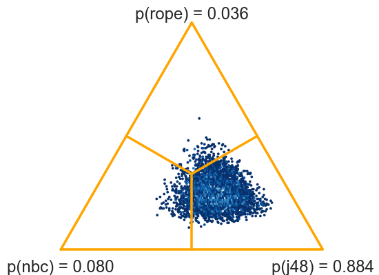
>>> two_on_multiple(nbc, j48, rope=1)
(0.23014, 0.00674, 0.76312)

There is 76.3 % probability that J48 is better than NBC.

>>> probs, fig = two_on_multiple(nbc, j48, rope=1, plot=True, names=names)
>>> fig.savefig("signedrank.png")

This test is computed from averages on data sets. We can also pass the entire data, that is, nbc and j48 as 54x10 matrices containing 10 scores for each of 54 data sets. The function will switch from signed-ranks test to a hierarchical model (Corani et al, 2015).

>>> probs, fig = two_on_multiple(nbc, j48, rope=1, plot=True, names=names)
(0.0795, 0.0365, 0.884)

If the results are obtained by multiple runs of cross validation, we must not forget to specify the number of runs.