Classes with tests¶

The two shortcut functions uses classes that actually prepare samples of posteriors, compute probabilities and plot the distributions.

Let nbc and j48 contain average performances of two methods for a collection of data sets. With shortcut functions, we computed the signed-ranks test with

>>> two_on_multiple(nbc, j48, rope=1)
(0.23014, 0.00674, 0.76312)

This is equivalent to calling SignedRankTest.probs:

>>> SignedRankTest.probs(nbc, j48, rope=1)
(0.23014, 0.00674, 0.76312)

We may choose a different test, the SignTest:

>>> SignTest.probs(nbc, j48, rope=1)
(0.26344, 0.13722, 0.59934)

To plot the distribution, we call

>>> fig = SignedRankTest.plot(nbc, j48, rope=1)

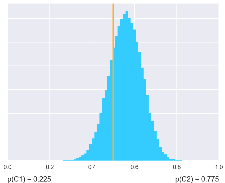
Or we may prefer to see as a histogram:

>>> fig = SignedRankTest.plot_histogram(nbc, j48, names=("nbc", "j48"))

Using test classes instead of shortcut functions offers more control and insight in what the tests do.

Single data set¶

The test for comparing two classifiers on a single data set is implemented in class CorrelatedTTest.

The class uses a Bayesian interpretation of the t-test (A Bayesian approach for comparing cross-validated algorithms on multiple data sets, G. Corani and A. Benavoli, Mach Learning 2015).

The test assumes that the classifiers were evaluated using cross validation. The number of folds is determined from the length of the vector of differences, as len(diff) / runs. Computation includes a correction for underestimation of variance due to overlapping training sets (Inference for the Generalization Error, C. Nadeau and Y. Bengio, Mach Learning 2003).

class baycomp.CorrelatedTTest(x, y, rope=0, runs=1, *, names=None, nsamples=50000)[source]¶

Compute and plot a Bayesian correlated t-test

classmethod compute_statistics(x, y, runs=1)[source]¶

Compute statistics (mean, variance) from the differences.

The number of runs is needed to compute the Nadeau-Bengio correction for underestimated variance.

Parameters:

x (np.array) – a vector of scores for the first model
y (np.array) – a vector of scores for the second model
runs (int) – number of repetitions of cross validation (default: 1)

Returns:

mean, var, degrees_of_freedom

classmethod sample(x, y, runs=1, *, nsamples=50000)[source]¶

Return a sample of posterior distribution for the given data

Parameters:

x (np.array) – a vector of scores for the first model
y (np.array) – a vector of scores for the second model
runs (int) – number of repetitions of cross validation (default: 1)
nsamples (int) – the number of samples (default: 50000)

Returns:

mean, var, degrees_of_freedom

classmethod probs(x, y, rope=0, runs=1)[source]¶

Compute and return probabilities

Probabilities are not computed from a sample posterior but from cumulative Student distribution.

Parameters:

x (np.array) – a vector of scores for the first model
y (np.array) – a vector of scores for the second model
rope (float) – the width of the region of practical equivalence (default: 0)
runs (int) – number of repetitions of cross validation (default: 1)

Returns:

(p_left, p_rope, p_right) if rope > 0; otherwise (p_left, p_right).

classmethod plot(x, y, rope=0, runs=1, *, names=None)[source]¶

Plot the posterior Student distribution as a histogram.

Parameters:

x (np.array) – a vector of scores for the first model
y (np.array) – a vector of scores for the second model
rope (float) – the width of the region of practical equivalence (default: 0)
names (tuple of str) – names of classifiers

Returns:

matplotlib figure

Multiple data sets¶

The library has three tests for comparisons on multiple data sets: a sign test (SignTest), a signed-rank test (SignedRankTest) and a hierarchical t-test (HierarchicalTest).

All classes have a common interface but differ in the computation of the posterior distribution. Consequently, some tests have specific additional parameters.

Common methods¶

The common behaviour of all tests is defined in the class Test.

class baycomp.multiple.Test(x, y, rope=0, *, nsamples=50000, random_state=None, **kwargs)[source]¶

classmethod sample(x, y, rope=0, nsamples=50000, **kwargs)[source]¶

Compute a sample of posterior distribution.

Derived classes override this method to implement specific sampling methods. Derived methods may have additional arguments.

Parameters:

x (np.array) – a vector of scores for the first model
y (np.array) – a vector of scores for the second model
rope (float) – the width of the region of practical equivalence (default: 0)
nsamples (int) – the number of samples (default: 50000)

Returns:

np.array of shape (nsamples, 3)

classmethod probs(x, y, rope=0, *, nsamples=50000, **kwargs)[source]¶

Compute and return probabilities

Parameters:

x (np.array) – a vector of scores for the first model
y (np.array) – a vector of scores for the second model
rope (float) – the width of the region of practical equivalence (default: 0)
nsamples (int) – the number of samples (default: 50000)

Returns:

(p_left, p_rope, p_right) if rope > 0; otherwise (p_left, p_right).

classmethod plot(x, y, rope, *, nsamples=50000, names=None, **kwargs)[source]¶

Plot the posterior distribution.

If there are samples in which the probability of rope is higher than 0.1, the distribution is shown in a simplex (see plot_simplex), otherwise as a histogram (plot_histogram).

Parameters:

x (np.array) – a vector of scores for the first model
y (np.array) – a vector of scores for the second model
rope (float) – the width of the region of practical equivalence (default: 0)
nsamples (int) – the number of samples (default: 50000)
names (tuple of str) – names of classifiers

Returns:

matplotlib figure

classmethod plot_simplex(x, y, rope, *, nsamples=50000, names=None, **kwargs)[source]¶

Plot the posterior distribution in a simplex.

The distribution is shown as a triangle with regions corresponding to first classifier having higher scores than the other by more than rope, the second having higher scores, or the difference being within the rope.

Parameters:

x (np.array) – a vector of scores for the first model
y (np.array) – a vector of scores for the second model
nsamples (int) – the number of samples (default: 50000)
names (tuple of str) – names of classifiers

Returns:

matplotlib figure

classmethod plot_histogram(x, y, *, nsamples=50000, names=None, **kwargs)[source]¶

Plot the posterior distribution as histogram.

Parameters:

x (np.array) – a vector of scores for the first model
y (np.array) – a vector of scores for the second model
nsamples (int) – the number of samples (default: 50000)
names (tuple of str) – names of classifiers

Returns:

matplotlib figure

Note that all methods are class methods. Classes are used as nested namespace. As described in the next section, it is impossible to construct an instance of a Test or derived classes.

Tests¶

class baycomp.SignTest(x, y, rope=0, *, nsamples=50000, random_state=None, **kwargs)[source]¶

Compute a Bayesian sign test (A Bayesian Wilcoxon signed-rank test based on the Dirichlet process, A. Benavoli et al, ICML 2014).

Argument prior can give a strength (as float) of a prior put on the rope region, or a tuple with prior’s position and strength, for instance (SignTest.LEFT, 1.0). Position can be SignTest.LEFT, SignTest.ROPE or SignTest.RIGHT.

class baycomp.SignedRankTest(x, y, rope=0, *, nsamples=50000, random_state=None, **kwargs)[source]¶

Compute a Bayesian signed-rank test (A Bayesian Wilcoxon signed-rank test based on the Dirichlet process, A. Benavoli et al, ICML 2014).

Arguments x and y should be one-dimensional arrays with average performances across data sets. These can be obtained using any sampling method, not necessarily cross validation.

class baycomp.HierarchicalTest(x, y, rope=0, *, nsamples=50000, random_state=None, **kwargs)[source]¶

Compute a hierarchical t test. (Statistical comparison of classifiers through Bayesian hierarchical modelling, G. Corani et al, Machine Learning, 2017).

Arguments x and y should be two-dimensional arrays; rows correspond to data sets and elements within rows are scores obtained by (possibly repeated) cross-validation(s).

The test is based on following hierarchical probabilistic model:

\[ \begin{align}\begin{aligned}\mathbf{x}_{i} & \sim MVN(\mathbf{1} \mu_i,\mathbf{\Sigma_i}),\\ \mu_1 ... \mu_q & \sim t (\mu_0, \sigma_0,\nu),\\ \sigma_1 ... \sigma_q & \sim \mathrm{unif} (0,\bar{\sigma}),\\\nu & \sim \mathrm{Gamma}(\alpha,\beta),\end{aligned}\end{align} \]

where \(q\) and \(i\) are the number of datasets and the number of measurements, respectively, and

\[ \begin{align}\begin{aligned}\alpha & \sim \mathrm{unif} (\underline{\alpha},\overline{\alpha}),\\\beta & \sim \mathrm{unif} (\underline{\beta}, \overline{\beta}),\\\mu_0 & \sim \mathrm{unif} (-1, 1),\\\sigma_0 & \sim \mathrm{unif} (0, \overline{\sigma_0}).\end{aligned}\end{align} \]

Parameters \(\underline{\alpha}\), \(\bar{\alpha}\), \(\underline{\beta}\), \(\bar{\beta}\) and \(\bar{\sigma_0}\) can be set through keywords arguments. Defaults are lower_alpha=1, upper_alpha=2, lower_beta = 0.01, upper_beta = 0.1, upper_sigma=1000.